Markov Chain Monte Carlo methods
MCMC methods can be used to estimate the posterior in an efficient way
In MCMC, the goal is to generate chains that after some iterations start sampling from the posterior
The posterior densities are then obtained in a Monte Carlo way:
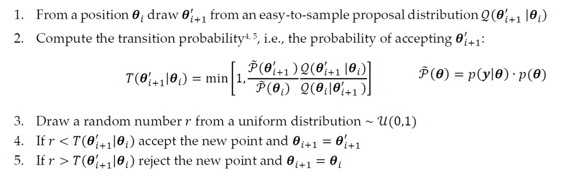
A popular approach for MCMC is the Metropolis-Hastings algorithm:
Optional 💽
🖱️Right-click and select “Save link as” to download the exercise HERE 👈 so you can work on it locally on your computer
Hint
Tips for working with emcee
Tuning algorithm:
Rule of thumb:
Make sure that the likelihood is supported in the entire prior domain (not ‘nans’)
Convergence:
We define a burn-in phase to discard samples still correlated to initial points
Number of initial samples (burn-in phase) Difficult to define a priori
Always check with Trace plots
Once converged, only a few steps (e.g. 100) are needed for most relevant metrics
Advanced topics:
Imports
import matplotlib.pyplot as plt
import numpy as np

# Problem definition
from probeye.definition.inverse_problem import InverseProblem
from probeye.definition.forward_model import ForwardModelBase
from probeye.definition.distribution import Normal, Uniform
from probeye.definition.sensor import Sensor
from probeye.definition.likelihood_model import GaussianLikelihoodModel
from probeye.definition.correlation_model import ExpModel

# Inference
from probeye.inference.emcee.solver import EmceeSolver

# Postprocessing
from probeye.postprocessing.sampling_plots import create_pair_plot
from probeye.postprocessing.sampling_plots import create_posterior_plot
from probeye.postprocessing.sampling_plots import create_trace_plot
Problem setup
# Fixed parameters
I = 1e9  # mm^4
L = 10_000  # mm

# Measurements
x_sensors = [2500, 5000]  # mm  (always from lower to higher, bug in inv_cov_vec_1D in tripy)
d_sensors = [35, 50]  # mm
sigma_model = 2.5  # mm
pearson = 0.5
l_corr = -np.abs(x_sensors[1] - x_sensors[0]) / np.log(pearson)  # mm (assuming exponential correlation)

# Prior
E_mean = 60  # GPa
E_std = 20  # GPa
Q_mean = 60  # kN
Q_std = 30  # kN
Q_loc_low = 0  # mm
Q_loc_high = 10000  # mm
Define forward model
def beam_deflection(E, Q, a, x):  # a is load position, x is sensor position
    if x < a:
        b = L - a
        return Q * b * x * (L ** 2 - b ** 2 - x ** 2) / (6 * E * I * L)

    return Q * a * (L - x) * (2 * L * x - x ** 2 - a ** 2) / (6 * E * I * L)
## Write your code where the three dots are
class BeamModel(ForwardModelBase):
def interface(self):
self.parameters = ...
self.input_sensors = Sensor("x")
self.output_sensors = Sensor("y", std_model="sigma")
def response(self, inp: dict) -> dict:
return {...}Define inverse problem
## Write your code where the three dots are

# Instantiate the inverse problem
problem = InverseProblem(...)

# Add latent parameters
problem.add_parameter(
    ...
)
problem.add_parameter(
    ...
)
problem.add_parameter(
  ...
)

# Add fixed parameters
problem.add_parameter(
 ...
)
problem.add_parameter(
...
)

# Add measurement data
problem.add_experiment(
...
)

# Add forward model
problem.add_forward_model(...)

# Add likelihood model
likelihood_model = GaussianLikelihoodModel(
        ...
        )
problem.add_likelihood_model(likelihood_model)
Solve with MCMC
emcee_solver = EmceeSolver(problem, show_progress=True)
inference_data = emcee_solver.run(n_steps=2000, n_initial_steps=2000)
Posterior plot
post_plot_array = create_posterior_plot(
    inference_data,
    emcee_solver.problem,
    kind="kde",
    title="Kernel density estimate of the posterior distribution",
)
Pair plot
pair_plot_array = create_pair_plot(
    inference_data,
    emcee_solver.problem,
    focus_on_posterior=True,
    show_legends=True,
    title="Pair plot of the posterior distribution",
)
Trace plot
## Write your code where the three dots are
trace_plot_array = create_trace_plot(
...
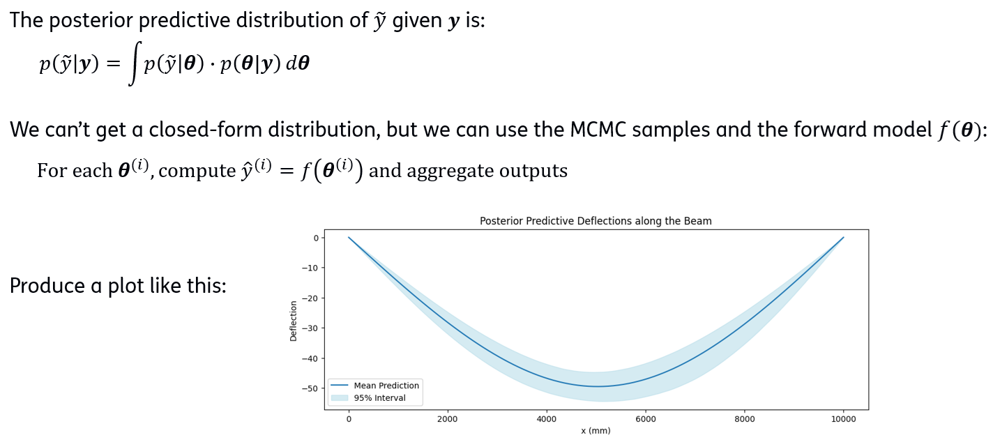
)Posterior predictives
## Write your code where the three dots are

 # Extract samples
posterior_samples = inference_data.posterior.to_array()  # parameters, chains, samples
posterior_samples = np.array(posterior_samples)
posterior_samples = posterior_samples.reshape(posterior_samples.shape[0], -1).T  # samples, parameters

# Make predictions for x in the range of the beam
x_range = np.linspace(0, 10000, 100)
predictions = np.zeros((len(posterior_samples), len(x_range)))

for i, sample in enumerate(posterior_samples):
    ...

# Calculate mean and 95% intervals
mean_pred = ...
lower_bound = ...  # 2.5th percentile
upper_bound = ...  # 97.5th percentile
Plot posterior predictive
plt.figure(figsize=(12, 4))
plt.plot(x_range, -mean_pred, label='Mean Prediction')
plt.fill_between(x_range, -lower_bound, -upper_bound, color='lightblue', alpha=0.5, label='95% Interval')
plt.xlabel('x (mm)')
plt.ylabel('Deflection')
plt.title('Posterior Predictive Deflections along the Beam')
plt.legend()
plt.show()
Complete Code! 📃💻
Here’s the complete code that you would run in your PC:
import matplotlib.pyplot as plt
import numpy as np

# Problem definition
from probeye.definition.inverse_problem import InverseProblem
from probeye.definition.forward_model import ForwardModelBase
from probeye.definition.distribution import Normal, Uniform
from probeye.definition.sensor import Sensor
from probeye.definition.likelihood_model import GaussianLikelihoodModel
from probeye.definition.correlation_model import ExpModel

# Inference
from probeye.inference.emcee.solver import EmceeSolver

# Postprocessing
from probeye.postprocessing.sampling_plots import create_pair_plot
from probeye.postprocessing.sampling_plots import create_posterior_plot
from probeye.postprocessing.sampling_plots import create_trace_plot

# Fixed parameters
I = 1e9  # mm^4
L = 10_000  # mm

# Measurements
x_sensors = [2500, 5000]  # mm  (always from lower to higher, bug in inv_cov_vec_1D in tripy)
d_sensors = [35, 50]  # mm
sigma_model = 2.5  # mm
pearson = 0.5
l_corr = -np.abs(x_sensors[1] - x_sensors[0]) / np.log(pearson)  # mm (assuming exponential correlation)

# Prior
E_mean = 60  # GPa
E_std = 20  # GPa
Q_mean = 60  # kN
Q_std = 30  # kN
Q_loc_low = 0  # mm
Q_loc_high = 10000  # mm


def beam_deflection(E, Q, a, x):  # a is load position, x is sensor position
    if x < a:
        b = L - a
        return Q * b * x * (L ** 2 - b ** 2 - x ** 2) / (6 * E * I * L)

    return Q * a * (L - x) * (2 * L * x - x ** 2 - a ** 2) / (6 * E * I * L)


class BeamModel(ForwardModelBase):
    def interface(self):
        self.parameters = ["E", "Q", "a"]
        self.input_sensors = Sensor("x")
        self.output_sensors = Sensor("y", std_model="sigma")

    def response(self, inp: dict) -> dict:
        E = inp["E"]
        Q = inp["Q"]
        a = inp["a"]
        x = inp["x"]
        return {"y": [beam_deflection(E, Q, a, float(x[0])), beam_deflection(E, Q, a, float(x[1]))]}  # float() needed, probably a bug in probeye


# Instantiate the inverse problem
problem = InverseProblem("Beam model with two sensors", print_header=False)

# Add latent parameters
problem.add_parameter(
    "E",
    tex="$E$",
    info="Elastic modulus of the beam (GPa)",
    prior=Normal(mean=E_mean, std=E_std),
)
problem.add_parameter(
    "Q",
    tex="$Q$",
    info="Load applied to the beam (kN)",
    prior=Normal(mean=Q_mean, std=Q_std),
)
problem.add_parameter(
    "a",
    tex="$a$",
    info="Position of the load (mm)",
    prior=Uniform(low=Q_loc_low, high=Q_loc_high)
)

# Add fixed parameters
problem.add_parameter(
    "sigma",
    tex="$\sigma$",
    info="Standard deviation of the model error (mm)",
    value=sigma_model,
)
problem.add_parameter(
    "l_corr",
    tex="$l_{corr}$",
    info="Correlation length of the model error (mm)",
    value=l_corr,
)

# Add measurement data
problem.add_experiment(
    name="TestSeries_1",
    sensor_data={"x": x_sensors, "y": d_sensors}
)

# Add forward model
problem.add_forward_model(BeamModel("BeamModel"), experiments="TestSeries_1")

# Add likelihood model
likelihood_model = GaussianLikelihoodModel(
        experiment_name="TestSeries_1",
        model_error="additive",
        correlation=ExpModel(x="l_corr")
        )
problem.add_likelihood_model(likelihood_model)

#solve mcmc
emcee_solver = EmceeSolver(problem, show_progress=True)
inference_data = emcee_solver.run(n_steps=2000, n_initial_steps=2000)


#posterior plot
post_plot_array = create_posterior_plot(
    inference_data,
    emcee_solver.problem,
    kind="kde",
    title="Kernel density estimate of the posterior distribution",
)

#pair plot
pair_plot_array = create_pair_plot(
    inference_data,
    emcee_solver.problem,
    focus_on_posterior=True,
    show_legends=True,
    title="Pair plot of the posterior distribution",
)

#trace plot
trace_plot_array = create_trace_plot(
    inference_data,
    emcee_solver.problem,
    title="Trace plot of the posterior distribution",
)

#Posterior predictives
# Extract samples
posterior_samples = inference_data.posterior.to_array()  # parameters, chains, samples
posterior_samples = np.array(posterior_samples)
posterior_samples = posterior_samples.reshape(posterior_samples.shape[0], -1).T  # samples, parameters

# Make predictions for x in the range of the beam
x_range = np.linspace(0, 10000, 100)
predictions = np.zeros((len(posterior_samples), len(x_range)))

for i, sample in enumerate(posterior_samples):
    E = sample[0]
    Q = sample[1]
    a = sample[2]
    predictions[i, :] = [beam_deflection(E, Q, a, x) for x in x_range]

# Calculate mean and 95% intervals
mean_pred = np.mean(predictions, axis=0)
lower_bound = np.percentile(predictions, 2.5, axis=0)
upper_bound = np.percentile(predictions, 97.5, axis=0)


#Plot posterior predictive

plt.figure(figsize=(12, 4))
plt.plot(x_range, -mean_pred, label='Mean Prediction')
plt.fill_between(x_range, -lower_bound, -upper_bound, color='lightblue', alpha=0.5, label='95% Interval')
plt.xlabel('x (mm)')
plt.ylabel('Deflection')
plt.title('Posterior Predictive Deflections along the Beam')
plt.legend()
plt.show()