Key Concepts - Crash course Bayesian system identification

The heart of Bayesian inference is Bayes’ theorem, which takes this form for continuous variables:

p(\boldsymbol{\theta}|\boldsymbol{y}) = \frac{p(\boldsymbol{y}|\boldsymbol{\theta}) \cdot p(\boldsymbol{\theta})}{\int p(\boldsymbol{y}|\boldsymbol{\theta}) \cdot p(\boldsymbol{\theta}) \, d\boldsymbol{\theta}}

or more intuitively:

\text{Posterior} = \frac{\text{Likelihood} \times \text{Prior}}{\text{Evidence}}

Parameters ( $\boldsymbol{\theta}$ ): The unknown system properties we want to identify
Measurements ( $\boldsymbol{y}$ ): Noisy sensor data from the system
Prior $p(\boldsymbol{\theta})$ : Parameter probabilities we assign before seeing data
Likelihood $p(\boldsymbol{y}|\boldsymbol{\theta})$ : Probability of observing the data given parameters
Posterior $p(\boldsymbol{\theta}|\boldsymbol{y})$ : Updated parameter knowledge after seeing data

Methods for Bayesian inference¶

Bayesian inference methods can be categorized based on their computational approach:

Exact methods: Conjugate priors provide analytical solutions when prior and posterior distributions belong to the same family
Exact methods (if run long enough): Numerical integration and sampling methods (MCMC, Nested sampling) that converge to exact solutions given sufficient computational time
Approximate methods: Variational inference and likelihood-free methods that provide fast approximations to the posterior

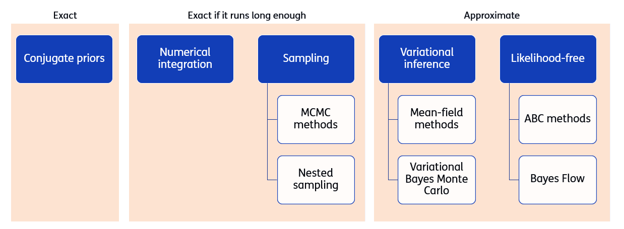
Note: Approximate methods are not covered in this crash course.

Some applications of Bayesian inference to structural engineering are:

Updating the resistance of a structure after passing a proof load test
Updating the reliability of a structure after it has survived a number of years
Updating the deterioration distribution on a structure after detecting corrosion in some areas
Updating the parameters of a finite element model after sensor data

The last application is known as system identification. Other names for it are Model updating and Model calibration.