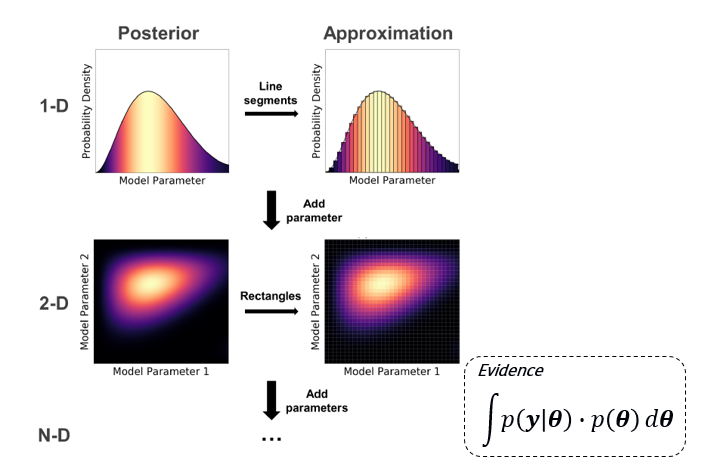
3. Numerical integration - Crash course Bayesian system identification

Numerical integration is straightforward to implement; however, “the curse of dimensionality” exists. This can be expressed mathematically as:

$n_{\text{points}} \sim \prod_{j=1}^{d} n_{\text{grids}} = n_{\text{grids}}^{d}$

where:

$n_{\text{points}}$ : Represents the number of points.
$\prod_{j=1}^{d} n_{\text{grids}}$ : Indicates the product of $n_{\text{grids}}$ from $j=1$ to $d$ .
$n_{\text{grids}}^{d}$ : Shows that the number of grids is raised to the power of $d$ .

numerical integration example — “A Conceptual Introduction to Markov Chain Monte Carlo Methods”, Joshua Speagle (2019)

Exercise 3

Estimate the elastic modulus ( $E$ ) of a simply supported bean from a measured deflection ( $\delta_\text{measured}$ )

Assume that we know the following:

The measurement uncertainty of deflection follows a normal distribution with zero mean and 1 cm standard deviation.
The measurement uncertainty is additive:

$\delta_\text{measured} = \delta_\text{real} + \text{measurement}_\text{unc}$

We have a single deflection measurement: $\delta_\text{measured} = 5$ cm.
The second moment of area (flexural inertia) of the beam is known, I = $1×10^5$ $\text{cm}^4$ .
The span of the beam is known, L = 10 m.
The self weight of the beam can be neglected, and it is loaded solely by a point load at the midspan with intensity, Q = 100 kN.
Bernoulli-Navier beam theory dis applicable, the material is linear elastic, the hinges at bot ends are perfec/idealized

Questions¶

What material is the beam made of?
How large is the elastic modulus of the beam?
Calculate the posterior of E.

Assume a normal distribution on E as prior with small information content (flat prior with a huge standard deviation).

Optional 💽

🖱️Right-click and select “Save link as” to download the exercise HERE 👈 so you can work on it locally on your computer

Hint

Start with formulating the likelihood function! Useful formulas for simple beams.

Prior $E$ $\approx$ $N(60,20)$ GPa

$\delta_{max} = \frac{QL^3}{48EI}$

The measurement error is obtained by the following formula:

$\delta_{𝑒𝑟𝑟𝑜𝑟,𝑖} = 50 - \frac{QL^3}{48E_iI}$

For a given $𝐸_𝑖$ , the probability density of having a measurement $\delta_{measured}$ = 50 is the probability density of the normal distribution with mean 0 and standard deviation 1, evaluated at $\delta_{𝑒𝑟𝑟𝑜𝑟,𝑖}$

Imports¶

import matplotlib.pyplot as plt
import numpy as np
from scipy import stats

Problem setup¶

# Fixed parameters
I = 1e9  # mm^4
L = 10_000  # mm
Q = 100  # kN

# Measurements
d_meas = 50  # mm
sigma_meas =  10  # mm

# Prior
E_mean = 60  # GPa
E_std = 20  # GPa

Forward model¶

def midspan_deflection(E):
    return Q * L ** 3 / (48 * E * I)

Bayesian functions¶

## Write your code where the three dots are

def likelihood(E):
    return ...


def prior(E):
    return ...

Perform numerical integration¶

## Write your code where the three dots are

E_values = np.linspace(-20, 140, 1000)

# Calculate prior and likelihood values
prior_values = ...
likelihood_values = ...

evidence = ... # use the trapezoidal rule to integrate
posterior_values = ...

Posterior summary¶

Hint

$P(A|B) = \frac{P(B|A) \cdot P(A)}{P(B)}$

CDF:

$F(A|B) = \left[ \sum_{j=1}^{i}P(A|B)_j \right ] \left(A_i-A_{i-1}\right)$

Mean:

$E(A|B) = \int A\cdot P(A|B)dA$

Standard deviation:

$\sigma(A|B) = \sqrt{\text{Var}(A|B)}$

$\text{Var}(A|B) = \int \left(A-E(A|B)\right)^2 \cdot P(A|B)dA$

## Write your code where the three dots are

 # Mean
mean = ... # use the trapezoidal rule to integrate
print(f'Mean: {mean:.2f} GPa')

# Median
cdf = np.cumsum(posterior_values) * np.diff(E_values, prepend=0)
median = E_values[np.argmin(np.abs(cdf - 0.5))]
print(f'Median: {median:.2f} GPa')

# Standard deviation
std = ...  # use the trapezoidal rule to integrate
print(f'Standard deviation: {std:.2f} GPa')

# 5th and 95th percentiles
percentiles = np.interp([0.05, 0.95], cdf, E_values)
print(f'5th percentile: {percentiles[0]:.2f} GPa')
print(f'95th percentile: {percentiles[1]:.2f} GPa')

Plot¶

plt.plot(E_values, prior_values, label='Prior')
plt.plot(E_values, likelihood_values, label='Likelihood')
plt.plot(E_values, posterior_values, label='Posterior')
plt.xlabel('E (GPa)')
plt.ylabel('Density')
plt.ylim([0, 0.045])
plt.legend()
plt.show()

Complete Code! 📃💻

Here’s the complete code that you would run in your PC:


import matplotlib.pyplot as plt
import numpy as np
from scipy import stats

# Fixed parameters
I = 1e9  # mm^4
L = 10_000  # mm
Q = 100  # kN

# Measurements
d_meas = 50  # mm
sigma_meas =  10  # mm

# Prior
E_mean = 60  # GPa
E_std = 20  # GPa

#forward model 
def midspan_deflection(E):
    return Q * L ** 3 / (48 * E * I)

def likelihood(E):
    return stats.norm.pdf(d_meas, loc=midspan_deflection(E), scale=sigma_meas)


def prior(E):
    return stats.norm.pdf(E, loc=E_mean, scale=E_std)

#numerical integration
E_values = np.linspace(-20, 140, 1000)
prior_values = prior(E_values)
likelihood_values = likelihood(E_values)

evidence = np.trapz(prior_values * likelihood_values, E_values)
posterior_values = prior_values * likelihood_values / evidence

#posterior summary
# Mean
mean = np.trapz(E_values * posterior_values, E_values)
print(f'Mean: {mean:.2f} GPa')

# Median
cdf = np.cumsum(posterior_values) * np.diff(E_values, prepend=0)
median = E_values[np.argmin(np.abs(cdf - 0.5))]
print(f'Median: {median:.2f} GPa')

# Standard deviation
std = np.sqrt(np.trapz((E_values - mean) ** 2 * posterior_values, E_values))
print(f'Standard deviation: {std:.2f} GPa')

# 5th and 95th percentiles
percentiles = np.interp([0.05, 0.95], cdf, E_values)
print(f'5th percentile: {percentiles[0]:.2f} GPa')
print(f'95th percentile: {percentiles[1]:.2f} GPa')

plt.plot(E_values, prior_values, label='Prior')
plt.plot(E_values, likelihood_values, label='Likelihood')
plt.plot(E_values, posterior_values, label='Posterior')
plt.xlabel('E (GPa)')
plt.ylabel('Density')
plt.ylim([0, 0.045])
plt.legend()