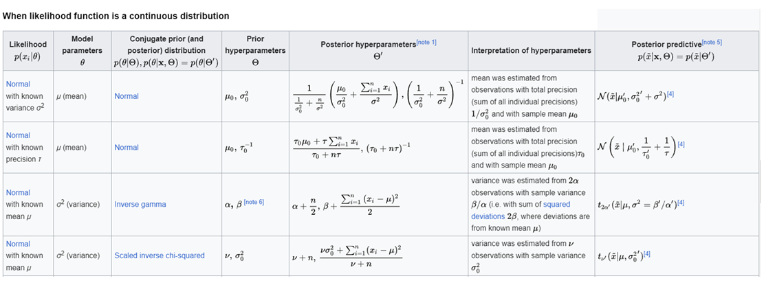
A conjugate prior is an algebraic convenience, giving a closed-form expression for the posterior; otherwise, numerical integration may be necessary.
More information about conjugate priors and tables of cojugate distribution can be found in wikipedia
Optional 💽
🖱️Right-click and select “Save link as” to download the exercise HERE 👈 so you can work on it locally on your computer
Hint
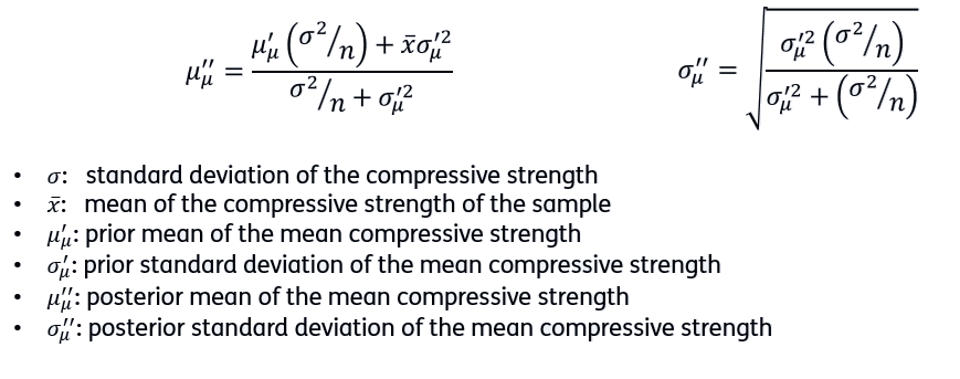
The compressive strength is normally distributed and its standard deviation σ is known, so if we assume that the prior distribution of the parameter µ (mean of the compressive strength) is normally distributed, then the posterior distribution remains Gaussian (conjugate). The mean and standard deviation of the posterior is defined as follows:
Import Necessary Libraries
We will start by importing the required libraries for our analysis.
import matplotlib.pyplot as plt
import numpy as np
from scipy import stats
Define Constants and Sample Data
Next, we define the constants, including the standard deviation and the sample data.
std = 5  # MPa
sample = [30.1, 28.7, 21.2, 28.6, 25.8, 25.1, 24.2, 27.3, 20.0, 34.8]  # MPa
n = len(sample)

prior_mu_mean = 40  # MPa
prior_mu_std = 100  # MPa
Calculate the Mean of the Sample
We calculate the mean of the sample data.
## Write your code where the three dots are
posterior_mu_mean = ...
print(f"Mean of the sample: {mean_sample:.2f} MPa")
Posterior Distribution with Conjugate Prior
Using the sample mean and the prior information, we calculate the posterior distribution.
## Write your code where the three dots are
posterior_mu_mean = ...
posterior_mu_std = ...
print(f"Posterior mean: {posterior_mu_mean:.2f} MPa")
print(f"Posterior standard deviation: {posterior_mu_std:.2f} MPa")
Mean of the sample: 26.58 MPa
Posterior mean: 26.58 MPa
Posterior standard deviation: 1.58 MPa
Plot the Distributions
## Write your code where the three dots are

x = np.linspace(0, 100, 1000)
prior = ...
posterior = ...

fig, ax = plt.subplots()
ax.plot(x, prior, label="Prior")
ax.plot(x, posterior, label="Posterior")
ax.set_xlim(0, 100)
ax.set_ylim(0, 0.3)
ax.set_xlabel("Mean (MPa)")
ax.set_ylabel("Density")
ax.set_title("Distribution of the Mean")
ax.legend()
plt.show()
Complete Code! 📃💻
Here’s the complete code that you would run in your PC:
import matplotlib.pyplot as plt
import numpy as np
from scipy import stats

std = 5  # MPa
sample = [30.1, 28.7, 21.2, 28.6, 25.8, 25.1, 24.2, 27.3, 20.0, 34.8]  # MPa
n = len(sample)

prior_mu_mean = 40  # MPa
prior_mu_std = 100  # MPa


# Calculate the mean of the sample
mean_sample = np.mean(sample)
print(f"Mean of the sample: {mean_sample:.2f} MPa")

# sttep 3 Posterior distribution with conjugate prior
posterior_mu_mean = (prior_mu_mean * (std ** 2 / n) + mean_sample * prior_mu_std ** 2) / (std ** 2 / n + prior_mu_std ** 2)
posterior_mu_std = np.sqrt(prior_mu_std ** 2 * (std ** 2 / n) / (prior_mu_std ** 2 + std ** 2 / n))
print(f"Posterior mean: {posterior_mu_mean:.2f} MPa")
print(f"Posterior standard deviation: {posterior_mu_std:.2f} MPa")

#plots
x = np.linspace(0, 100, 1000)
prior = stats.norm.pdf(x, prior_mu_mean, prior_mu_std)
posterior = stats.norm.pdf(x, posterior_mu_mean, posterior_mu_std)

fig, ax = plt.subplots()
ax.plot(x, prior, label="Prior")
ax.plot(x, posterior, label="Posterior")
ax.set_xlim(0, 100)
ax.set_ylim(0, 0.3)
ax.set_xlabel("Mean (MPa)")
ax.set_ylabel("Density")
ax.set_title("Distribution of the Mean")
ax.legend()
plt.show()